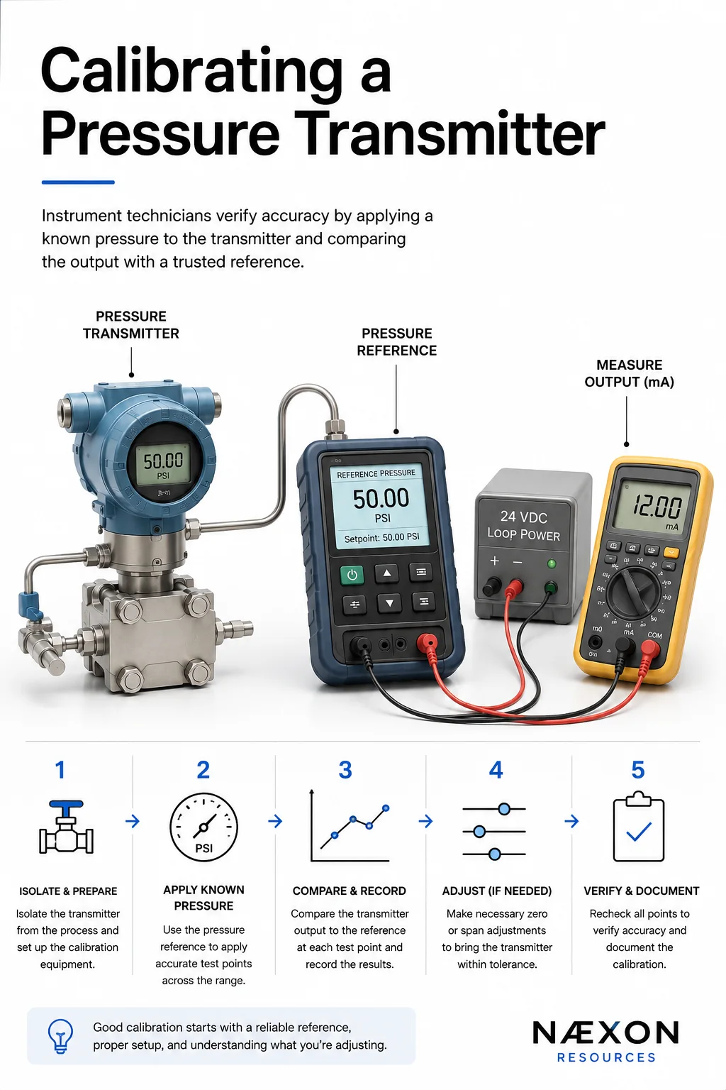
Pressure transmitters are everywhere in modern industrial facilities. Refineries, chemical plants, power plants, pipelines, compressor stations, manufacturing facilities, and other process plants rely on them to tell the control system what is happening inside equipment and piping.
A transmitter might be watching 25 psi of process pressure, 1,500 psi on a high-pressure system, differential pressure across a filter, or the pressure difference used to infer flow or vessel level. Whatever the application, the basic job is similar: sense pressure accurately and convert that measurement into a signal the control system can understand.
One of the most common arrangements is a transmitter producing a 4–20 mA signal. In a simple 0–100 psi example, 0 psi corresponds to 4 mA and 100 psi corresponds to 20 mA. Halfway through the calibrated range, 50 psi should correspond to approximately 12 mA.
Calibration is how an instrument technician verifies that those relationships are actually correct.
What Calibration Really Means
A common misconception is that calibrating a transmitter simply means connecting a communicator and pressing a calibration button.
The fundamental concept is much simpler.
The technician applies a known, accurate pressure to the transmitter. The transmitter reports what it believes that pressure is and, when applicable, produces a corresponding electrical output. The technician compares the transmitter’s response against the known reference.
If the reference says 50.000 psi while the transmitter reports 50.002 psi, the difference may be perfectly acceptable depending on the required tolerance. If the transmitter reports 52 psi, something is clearly wrong.
This distinction matters because verification and adjustment are not the same thing. Emerson describes pressure-transmitter calibration as comparing the transmitter against a known accurate applied pressure; if the difference is within the required tolerance, a sensor trim is not necessary. (Emerson.com)
A good instrument technician therefore doesn’t automatically adjust a transmitter just because it is connected to calibration equipment.
First, you determine whether it actually needs adjustment.
Understanding 4–20 mA Before Calibrating Anything
For a conventional linear 4–20 mA pressure transmitter, the electrical span is 16 mA.
That comes from:
20 mA − 4 mA = 16 mA
The lower end of the measurement range is represented by 4 mA, while the upper end is represented by 20 mA.
Imagine a transmitter configured for:
LRV = 0 psi
URV = 100 psi
Its ideal response would be:
0 psi = 4 mA
25 psi = 8 mA
50 psi = 12 mA
75 psi = 16 mA
100 psi = 20 mA
The important concept is percentage of span.
At 25 psi, the transmitter is at 25% of its calibrated pressure span. Twenty-five percent of the 16 mA electrical span is 4 mA. Add that to the 4 mA live-zero value and the expected output becomes 8 mA.
The general relationship for a linear transmitter is:
Output mA = 4 + [(Applied Pressure − LRV) ÷ (URV − LRV)] × 16
Understanding that equation makes troubleshooting much easier because the technician isn’t merely memorizing that 50% equals 12 mA. He understands why it equals 12 mA.
What the Instrument Technician Is Actually Testing
A pressure transmitter is essentially performing two conversions.
First, the pressure sensor interprets the physical pressure applied to it and converts that into a digital process measurement. Then, on an analog-output transmitter, the electronics convert that measurement into the corresponding 4–20 mA output.
Those two parts can develop different errors.
Suppose the technician applies exactly 50 psi.
The transmitter’s digital process variable says 48 psi, and the analog output corresponds correctly to that incorrect 48 psi measurement.
That points toward the pressure measurement side.
Now consider another situation. The technician applies exactly 50 psi and the digital process variable correctly reports 50 psi, but the actual loop current isn’t the expected 12 mA.
Now the sensor may be reading pressure correctly while the analog output side needs attention.
Modern smart transmitters allow technicians to distinguish between these problems instead of simply turning zero and span adjustments until the numbers look right. Emerson’s documentation specifically separates sensor trim from analog output trim for this reason. (Emerson.com)
The Basic Calibration Setup
A typical bench setup includes the pressure transmitter, an accurate pressure reference or pressure calibrator, a controlled pressure source such as a hand pump, the necessary tubing and fittings, loop power when required, and a way to accurately measure the transmitter’s current output.
Some modern pressure calibrators combine several of these functions. For example, equipment is available that can generate or measure pressure, measure 4–20 mA current, and provide 24 V loop power to the transmitter.
The reference instrument matters tremendously. You cannot prove that a transmitter is accurate by comparing it against an unknown or less suitable reference. For sensor trimming, Emerson’s Rosemount 2051 manual recommends a pressure input source at least three times more accurate than the transmitter being trimmed. (Emerson.com)
That principle applies throughout instrumentation:
Your calibration is only as trustworthy as your reference.
This same idea appears elsewhere in industrial work. Pressure gauges used during hydrostatic testing of industrial piping also need appropriate range and calibration status. Instrumentation takes that same measurement discipline much further.
Isolate the Transmitter Before Applying Test Pressure
In the field, the first major challenge isn’t pressing buttons on a calibrator. It is establishing a safe and correct test condition.
A transmitter connected to an operating process cannot simply be disconnected or pressurized however someone feels like doing it. The technician needs to understand the process, the manifold arrangement, the pressure source, the instrument’s rating, the facility procedure, and what the control system will do when the transmitter signal changes.
Depending on the application, operations may need to place the associated control loop in manual, bypass an alarm or interlock under an approved procedure, isolate the process connection, equalize a differential-pressure transmitter, or otherwise establish a safe calibration condition.
This is why instrumentation work requires more than knowing electronics.
The technician has to understand the process.
Opening the wrong manifold valve on a differential-pressure transmitter or disturbing an instrument connected to a live process can create consequences far beyond an inaccurate reading.
The same discipline applies whenever workers are dealing with stored pressure. Næxon’s guide to pneumatic testing of industrial piping explains why controlled pressure, proper boundaries, isolation, and line-of-fire awareness matter whenever pressurized systems are involved.
Verify the Transmitter’s Configuration
Before performing the actual calibration, the technician needs to know what the transmitter is supposed to do.
Assume the tag is PT-101.
The calibration documentation may show that PT-101 is ranged from 0 to 100 psi with a 4–20 mA output.
That means:
0 psi = 4 mA
and:
100 psi = 20 mA
But suppose somebody previously changed the transmitter configuration to 0–200 psi.
Now 100 psi should produce approximately 12 mA rather than 20 mA.
The transmitter might be operating perfectly according to its current configuration while still being completely wrong for the application.
That is why calibration isn’t merely a physical measurement exercise. Configuration has to agree with the approved instrument data.
Perform the As-Found Test First
One of the most important habits in calibration work is obtaining the as-found condition before making adjustments.
The as-found test tells you how the transmitter was actually performing when you arrived.
If you immediately perform a zero trim, sensor trim, or output adjustment, you destroy that information.
A common calibration sequence checks several points across the range. The exact number and sequence are determined by the site’s procedure, calibration standard, instrument requirements, and required accuracy. A basic example might include 0%, 25%, 50%, 75%, and 100% of range and then return downward through the range.
For our 0–100 psi example, that would mean checking pressures such as 0, 25, 50, 75, and 100 psi while observing the corresponding pressure reading and mA output.
Fluke’s calibration guidance similarly describes applying known pressures, reading both the reference pressure and transmitter current, and repeating the comparison across the required test points. (Fluke)
The technician records the results before touching the calibration.
That record can reveal much more than simply “pass” or “fail.”
Why Technicians Test Up and Down the Range
Imagine that the transmitter reads correctly as pressure increases but doesn’t return to the same readings as pressure decreases.
That difference can reveal behavior that a single zero-and-span check might miss.
Testing multiple points also helps reveal nonlinearity. A transmitter could look perfect at 0% and 100% while still being wrong in the middle.
This is why simply applying zero pressure, adjusting 4 mA, applying full pressure, adjusting 20 mA, and calling the instrument calibrated can be inadequate for precision instrumentation.
You want to know how the transmitter behaves throughout its working range.
Zero Trim Is Not the Same as Reranging
This is one of the most important concepts for someone learning smart transmitters.
Zero trim and reranging are different operations.
Suppose a transmitter is intended to measure 0–100 psi.
Reranging tells the transmitter:
“Treat 0 psi as the lower range value and 100 psi as the upper range value.”
A sensor trim tells the transmitter:
“The reference pressure being applied right now is the true pressure. Correct your measurement to agree with it.”
Those are not the same instruction.
Modern smart transmitters are factory characterized, so unnecessary or inaccurate trimming can actually make their performance worse. Emerson warns that improper trimming or trimming with inaccurate equipment can degrade transmitter performance. (Emerson.com)
That is why good technicians don’t “calibrate by button pushing.”
They determine what error exists first.
Understanding Zero Trim
Zero trim is a single-point sensor adjustment commonly used to compensate for a small zero offset, including certain mounting-position effects.
For a gauge-pressure transmitter, the instrument may be properly vented to atmosphere so the true applied gauge pressure is zero. If the transmitter reports a small nonzero pressure, an appropriate zero trim can correct that offset when permitted by the manufacturer’s procedure.
For a differential-pressure transmitter, establishing true zero requires the correct manifold condition. The technician needs both sides at the same pressure, not simply an assumption that the process is at zero.
Rosemount’s guidance describes venting or equalizing the transmitter before performing a zero trim and notes that mounting position can create a zero shift. (Emerson.com)
This becomes especially important with remote seals, wet legs, elevated or suppressed-zero applications, and other installations where “zero” does not necessarily mean an empty process connection sitting at atmospheric pressure.
Sensor Trim Goes Deeper
If the transmitter’s digital pressure measurement does not agree with the accurate reference pressure, the technician may need a sensor trim according to the manufacturer’s procedure.
A two-point sensor trim typically uses a lower and upper pressure reference.
The technician applies an accurately known lower pressure and tells the transmitter what that pressure truly is. Then an accurately known upper pressure is applied and identified.
The transmitter uses those reference points to correct its interpretation of the sensor.
This is why the quality of the pressure standard matters so much.
If you tell the transmitter that an inaccurate reference is correct, you aren’t calibrating the transmitter.
You’re teaching it the wrong answer.
Analog Output Trim Is a Different Adjustment Again
Now imagine that the pressure side is perfect.
You apply 50 psi.
The transmitter’s digital process variable says 50 psi exactly.
The configuration is 0–100 psi.
The transmitter therefore believes it should be producing 12.000 mA.
But your accurate current reference measures 11.940 mA.
That points toward the digital-to-analog output rather than the pressure sensor.
An analog output trim, sometimes called a 4–20 mA output trim or D/A trim depending on the device, aligns the actual current output with an accurate current reference. Emerson describes this separately from the pressure sensor trim. (Emerson.com)
Understanding this distinction is one of the things that separates actual instrumentation troubleshooting from simply adjusting numbers until everything appears correct.
Perform the As-Left Test
Once any necessary adjustment has been completed, the calibration isn’t finished.
The technician repeats the required test.
This creates the as-left condition.
The transmitter is again exercised through the specified test points and the results are documented. The final values have to satisfy the project’s required tolerance.
This gives the facility two valuable records.
The as-found data shows how the instrument was performing before intervention.
The as-left data shows how it was performing when the technician finished.
Those records can help maintenance and reliability teams identify drift, determine whether calibration intervals are appropriate, investigate process problems, and recognize instruments that repeatedly fall outside tolerance.
A Simple 0–100 PSI Example
Imagine PT-101 has a calibrated range of 0–100 psi.
At zero pressure, you expect approximately 4 mA.
At 25 psi, approximately 8 mA.
At 50 psi, approximately 12 mA.
At 75 psi, approximately 16 mA.
At 100 psi, approximately 20 mA.
Now apply an accurate 50 psi reference.
The transmitter reports 50.00 psi and the current meter reads 12.00 mA.
Excellent.
Now apply 100 psi.
The transmitter reports 100.00 psi and the current reads 20.00 mA.
Again, excellent.
There is no reason to adjust something simply because the calibration equipment is connected.
If all required test points are within the specified tolerance, the calibration verification may be complete.
That is an important lesson:
Calibration does not automatically mean adjustment.
What Happens When the Transmitter Passes but the Control Room Reading Is Wrong?
This is where instrumentation becomes especially interesting.
Suppose the technician proves that the transmitter is producing exactly 12.00 mA at 50% pressure, but the control system shows 46%.
The transmitter may not be the problem at all.
Now the troubleshooting moves into the loop.
The technician may investigate wiring, loop resistance, terminal condition, power supply, barriers or isolators, analog input scaling, PLC/DCS configuration, grounding issues, or another component between the transmitter and the control system.
A loop calibrator can also simulate a known 4–20 mA signal into downstream equipment. For example, feeding a known 12 mA signal into the input side can help determine whether the receiving system interprets 50% correctly. Fluke describes mA sourcing as a method for testing control-system input devices independently of the transmitter. (Fluke)
This is why replacing the transmitter every time the control room sees a bad number is poor troubleshooting.
First determine where the error begins.
Differential-Pressure Transmitters Require More Thinking
A differential-pressure transmitter measures the difference between its high-pressure and low-pressure sides.
If the high side sees 100 psi and the low side sees 90 psi, the transmitter sees:
100 − 90 = 10 psi differential pressure
That DP might represent flow across a primary element, level in a pressurized vessel, filter condition, or another process variable.
Calibrating the transmitter therefore requires understanding which port receives the reference pressure, how the opposite side is treated, what the manifold is doing, and what the transmitter’s configured differential range actually represents.
A technician who understands only “put pressure in and read milliamps” can get into trouble quickly.
Instrumentation requires understanding what the device is measuring physically.
Pressure Transmitter Calibration Is Really a Chain of Trust
Think about the entire measurement path.
The process creates pressure.
The sensing element detects it.
The transmitter electronics interpret it.
The transmitter communicates a digital value and/or converts that measurement into 4–20 mA.
The wiring carries the signal.
The control system receives it.
The input card interprets it.
The software scales it.
Finally, an operator sees a number on a screen.
Every link has to be right.
This is why instrument technicians are so important in refineries and process plants. Næxon’s guide to the highest-paying skilled trades in the oil and gas industry includes instrument technicians because modern facilities depend heavily on workers who can understand sensors, transmitters, electrical loops, calibration, process equipment, and control systems together.
The job isn’t simply turning a screwdriver.
It’s proving that a physical condition occurring somewhere inside a plant is being represented accurately several hundred feet—or sometimes several miles—away.
The Most Important Habit: Know What You Are Adjusting
If there is one concept worth remembering from pressure-transmitter calibration, it is this:
Don’t adjust an instrument until you understand what is wrong.
If the pressure reference and digital process variable disagree, investigate the pressure measurement side.
If the digital process variable is correct but the actual 4–20 mA output is wrong, investigate the analog output.
If both are correct but the DCS indication is wrong, investigate the loop and receiving system.
If everything is within tolerance, don’t create a problem by unnecessarily trimming a perfectly good transmitter.
That diagnostic thinking is the real skill.
Anyone can learn the button sequence on a communicator.
A good instrument technician understands what those buttons are actually changing—and knows when not to press them.
For more industrial training covering instrumentation, piping, welding, electrical work, refinery operations, rigging, millwright work, and other skilled trades, continue through the Næxon Resources & Learning Center.